
Having already identified the top 10 “rogue states” in our last Blog Post, this week we can now go on to analyze whether any payments have actually been made to a bank account in one of those dubious states and if so to what extent. So without further ado – let’s get down to business and get our hands dirty!
The basics of “rogue states”
Perhaps the term “rogue states” is completely foreign to you and you are not really sure what it means? If so, I recommend you take a look at the blog post from last week first. But for the more lazy readers out there, here’s a quick recap:
Various organizations deal with the classification of countries in terms of the extent of corruption. This is quite an extensive area, which is why the organizations have different priorities, such as money laundering, financing nuclear weapons or the like. For example, every year the non-governmental organization Transparency International publishes the Corruption Perception Index (CPI), a list of perceived levels of corruption. According to this index, the Scandinavian countries (Denmark, Norway, Sweden, Finland) are among the top 6 with the least perceived corruption. Germany is in 10th place, but it is really the other end of the list that we need to look at to serve as a basis for our analysis in SAP:
| Rank | Country | Score |
|---|---|---|
| 166 | Iraq | 17 |
| 166 | Venezuela | 17 |
| 168 | Guinea-Bissau | 16 |
| 169 | Afghanistan | 15 |
| 170 | Yemen | 14 |
| 170 | Libya | 14 |
| 170 | Sudan | 14 |
| 174 | North Korea | 12 |
| 175 | Southern Sudan | 11 |
| 176 | Somalia | 10 |
Now, of course, it depends on your company, your industry and your trade relations, but we would not normally want to be providing support for criminal activities in these countries with funds from our company. We have already identified the top 10 “rogue states”. So now let’s see how things look in SAP.
Data basis for the evaluation of payments to “rogue states”
Before we can carry out an analysis, we first need the relevant data for an evaluation. We obtain these from the SAP tables “REGUP” (Processed items from the payment program) and “REGUH” (Settlement data from payment program). The tables contain useful information, for example, on the bank code of the payee’s bank, the paying company code, but also the country key of the corresponding bank (REGUH table, fields: ZBNKL, ZBUKR and ZBNKS) or the document number of the paid invoice (REGUP table, field: BELNR). In addition, we are only interested in the actual payments and want to ignore all trial payment runs. This is what the field “XVORL” is for in REGUP and REGUH. This gives us the information we need about the relevant bank data in SAP that was used for payments.
However, we are also interested in the level of cash flows to dubious states. The relevant fields for the evaluation can also be found in the REGUP table:
- BUZEI (Number of Line Item Within Accounting Document)
- LIFNR (Account Number of Vendor or Creditor)
- SHKZG (Debit/credit indicator)
- DMBTR (Amount in local currency)
In addition to the amount of invoices paid and unpaid, it is also possible to determine the absolute number of invoices. If we put the individual pieces of the puzzle together for evaluation in the SQL Editor (SAP transaction: DBACOCKPIT – Diagnosis – SQL Editor), we obtain the following query (tested on a HANA database):
SELECT R.MANDT,P.BUKRS,P.GJAHR,ZBNKS BANKCOUNTRY,COUNT(DISTINCT P.BELNR) AMOUNT_INVOICES_PAID,SUM(CASE WHEN P.SHKZG=’H’ THEN P.DMBTR ELSE 0 END) SUM_CREDIT ,SUM(CASE WHEN P.SHKZG=’S’ THEN P.DMBTR ELSE 0 END) SUM_DEBIT, SUM(CASE WHEN P.SHKZG=’H’ THEN P.DMBTR ELSE 0 END)-SUM(CASE WHEN P.SHKZG=’S’ THEN P.DMBTR ELSE 0 END) SUM_PAID
FROM REGUH R JOIN REGUP P ON
(R.MANDT=P.MANDT AND R.LAUFD=P.LAUFD AND R.LAUFI=P.LAUFI AND R.ZBUKR=P.ZBUKR AND R.LIFNR=P.LIFNR AND P.VBLNR=R.VBLNR AND R.EMPFG=P.EMPFG AND ((R.XVORL IS NULL OR R.XVORL LIKE ”) AND (P.XVORL IS NULL OR P.XVORL LIKE ”)))
WHERE P.LIFNR NOT LIKE ” AND R.LIFNR NOT LIKE ” AND ZBNKS NOT LIKE ”
GROUP BY R.MANDT,P.BUKRS,P.GJAHR,ZBNKS
Don’t worry, the query is only a “SELECT” query, so that we only access the data in read-only. No data is changed in SAP, so that we can happily go ahead and execute the query using the “Execute (F8)” button. The result may look something like this:
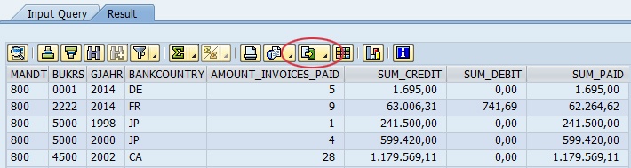
This makes it clear very quickly not only which countries payments have been made to (BANKCOUNTRY), but also how high the total liabilities were in the corresponding countries (SUM_CREDIT), how high the potential credits were (SUM_DEBIT) and how much of them have already been paid (SUM_PAID). Using the “Export – Spreadsheet” option (marked in red in the screenshot), we can also evaluate and visualize the results in Excel.
Further analysis in Excel
This is where we follow our standard procedure, which over the past weeks and months has become established as a tried-and-tested method of visualizing data in Excel: you guessed it, a chart generated from a pivot table.
After exporting the data to Excel, navigate to the “Insert – PivotTable” tab. Excel should then automatically select the table area, so that we simply have to confirm by clicking “OK”. For the PivotTable, we then select the following fields, for example:
- BANKCOUNTRY (as lines)
- AMOUNT_INVOICES_PAID (as values)
- SUM_PAID (as values)
Once that’s done, we can quickly insert a chart using “Insert – Charts – Insert Column Chart – Clustered Column” and then we are almost finished. In my example, there is an extremely large number of liabilities within Germany, which is why I will use a logarithmic scale to base 10 for the Y-axis. This means that extremely large numbers are relativized and become comparable to smaller values. In the result, only the ratio is displayed and not the absolute values, e.g. the value 100,000 becomes 5; the logarithm of ten becomes somewhat clearer with the representation of its inverse function:
y = 10X describes the inverse function and is therefore synonymous with x = log (y)
In concrete terms, that means:
Reverse function: 100,000 = 105
Logarithm: 5 = log (100,000)
You can apply this setting simply by clicking on the scale of the Y-axis and selecting “Axis Options” in the right window and selecting “Logarithmic scale”. Usually, base 10 is the default setting. My result will now look like this:
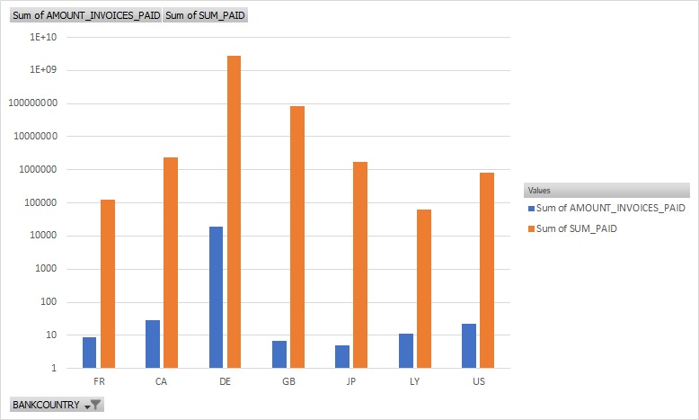
And lo and behold, what do we see? Right next to Japan (JP), there is one of Egypt’s neighbors: Libya (LY). To be totally honest with you, I had to check the country code LY too, because I had no idea what country it was supposed to stand for. Now let’s take a step back and take a look at our top 10 “rogue states”: Libya is ranked number 4 next to Sudan and Yemen. So we’ve really hit the bull’s-eye with that one then….and it’d certainly be worth taking a closer look unless you work for a well-known defense contractor, that is…?
Perhaps any talk of SQL, Queries or SELECT just leaves you plain baffled? Then why not let zap Audit do all the hard work of data analysis for you so that you can concentrate on what you do best: Auditing. After all, that is exactly what zap Audit is designed to do. Automated data analysis in SAP so that the auditor can focus on the essentials. Still having doubts? Then you can find quick and easy answers to any questions you may still have here:
If you don’t ask, you’ll never know.
Put your questions to us, contact us here!